Title: Exploration by Random Network Distillation
Authors
- Yuri Burda
- Harrison Edwards
- Amos Storkey
- Oleg Klimov
Prerequisites
- Proximal Policy Optimization Algorithms (Schulman et al., 2017) [Arxiv] [Paper]
- Curiosity-driven Exploration by Self-supervised Prediction (Pathak et al., 2017) [Arxiv] [Paper]
- Randomized Prior Functions for Deep Reinforcement Learning (Osband et al., 2018) [Arxiv] [Paper]
Accompanying Resources
- Implementation of RND in the ICLR2019 submission [Code]
- Large-Scale Study of Curiosity-Driven Learning (Burda et al., 2018) [Arxiv] [Paper]
This review was first presented the reading group of Reinforcement Learning Intelligence (RLI). Thank you to the members for helpful feedback.
1 Introduction
Reinforcement Learning works well when the reward function is dense and easy to find.
- Dense: A lot of rewards are nonzero.
- Easy to find: A random agent finds nonzero rewards.
However, reinforcement learning algorithms fail when the rewards are sparse and hard to find. One solution would be to hand-engineer dense reward functions. However, this is often impractical or impossible. Another solution is to develop more sophisticated exploration methods. Exploration methods have been a popular research topic, with a lot of new sophisticated methods with better results on hard exploration games. (Check my rl-exploration repository for an overview of exploration methods)
| Count-based | Curiosity |
|---|---|
| Unifying Count-Based Exploration and Intrinsic Motivation | Curiosity-driven Exploration by Self-supervised Prediction |
| Count-Based Exploration with Neural Density Models | Large-Scale Study of Curiosity-Driven Learning |
However, these exploration methods are difficult to scale up: due to their complexity, it is difficult to deploy them in parallel environments. This is a crucial problem, since recent state of the art methods rely on using parallel environments to collect large number of samples. In contrast, we propose an approach called Random Network Distillation (hereafter RND) that is simpler to implement, works with high-dimensional observations, can be incorporated with policy optimization algorithms, and efficient.
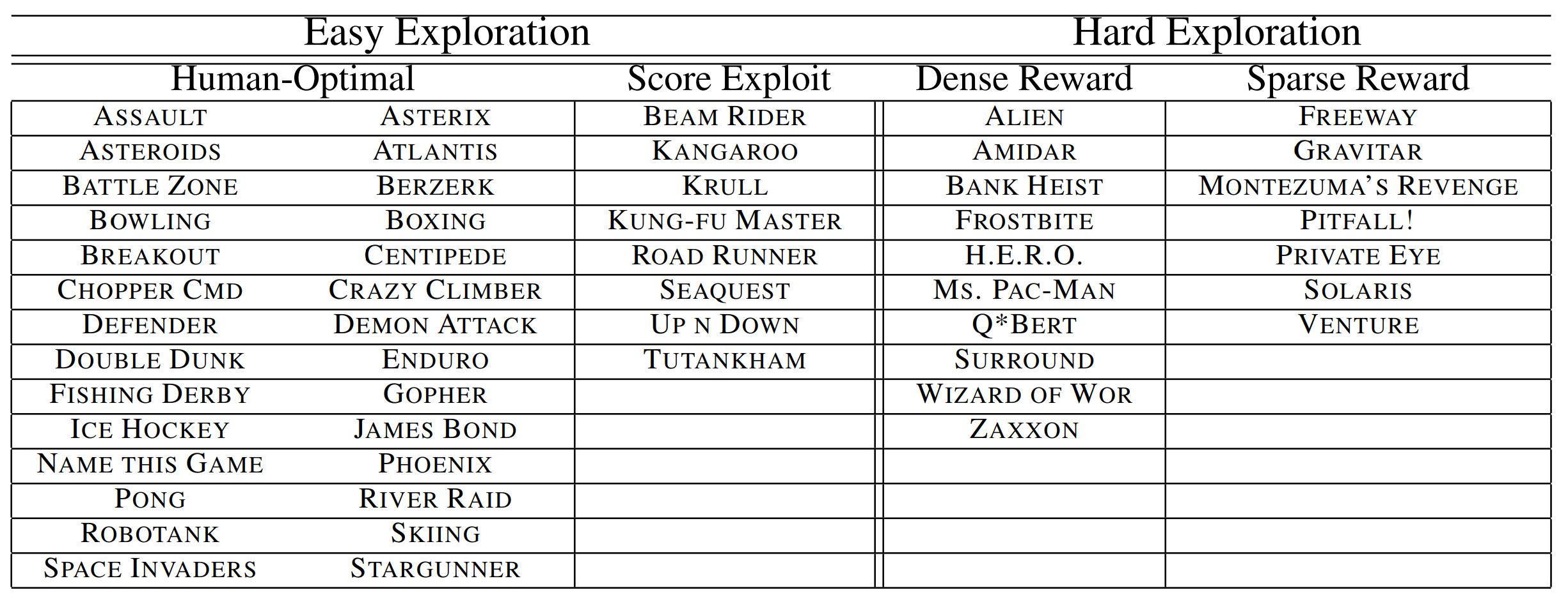
We experiment with RND on selected Atari 2600 games, a standard benchmark for deep reinforcement learning algorithms. We select hard exploration games with sparse rewards: Freeway, Gravitar, Montezuma’s Revenge, Pitfall!, Private Eye, Solaris, and Venture.
Combined with PPO, RND achieves state-of-the-art performance in Montezuma’s Revenge, periodically finds all 24 rooms and solves the first level without using demonstrations or having access to the underlying state of the game.
2 Method
2.1 Exploration Bonuses
Exploration bonuses are a class of methods that encourages exploration even when the reward $e_t$ is sparse. This is done by augmenting $e_t$ to create a new reward $r_t = e_t + i_t$, where $i_t$ is the exploration bonus associated with the transition at time $t$. The reward given by the environment is often called the extrinsic reward, and the augmented reward is called the intrinsic reward.
To encourage exploration, the intrinsic reward $i_t$ should be designed so that it is high in novel states than in frequently visited states. In a tabular setting with a finite number of states, this is easy: we can simply count the number of visits at each state. Then, we can define $i_t$ as a decreasing function of the visitation count $n(s)$. These are called count-based exploration methods.
\(i_t = \frac{\beta}{n(s)}, \frac{\beta}{\sqrt{n(s)}}\) In non-tabular cases, it is difficult to define counts, as most states are visited at most once. A possible generalization is to use define a pseudo-count, using state density estimates $N(s)$ as an exploration bonus. Using density estimates, even states that have never been visited have positive pseudo-count if it is similar to other visited states.
Another way to design the intrinsic reward $i_t$ is to define it with a prediction error for a problem related to the agent’s transitions.
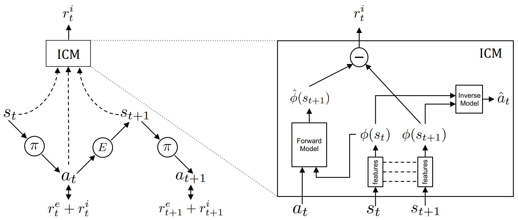
The most relevant example would be the Intrinsic Curiosity Module (Pathak et al., 2017; Burda et al., 2018). The Intrinsic Curiosity Module (hereafter ICM) trains forward model that outputs a prediction $\hat{\phi}(s_{t+1})$ that attempts to predict the encoded next state $\phi(s_{t+1})$ given encoded state $\phi(s_t)$ and action $a_t$. The intrinsic reward $r^i_t$ is defined as the prediction error of the forward model. The forward model is trained as the agent explores the environment. Thus, low prediction error means that the ICM has understood the transition $(s_t, a_t)$.
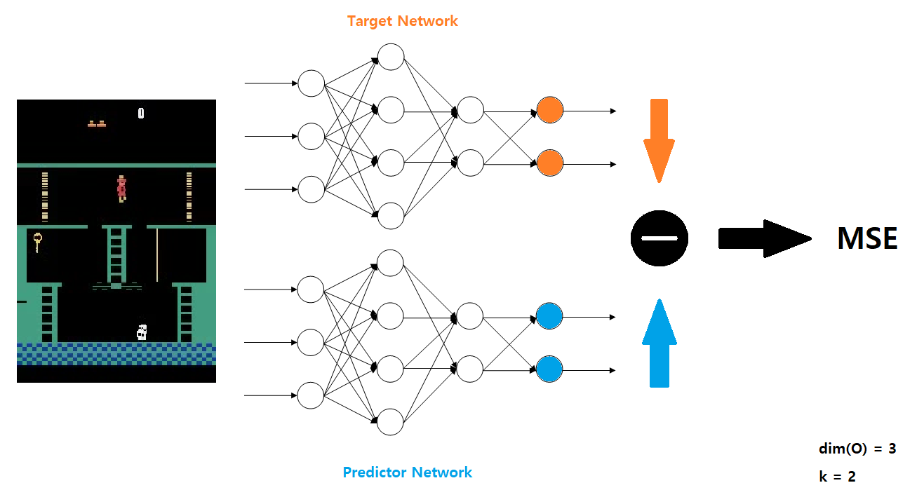
2.2 Random Network Distillation
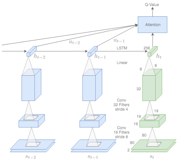
We introduce Random Network Distillation (RND), a state-based prediction-error-based exploration method. We define two networks: a target network $f$ and a predictor network $\hat{f}$. The target network is fixed after random initialization, and is the target of the prediction problem.The predictor network trains on the data collected by the agent to solve the prediction problem. In other words, with the data collected by the agent, the predictor network $\hat{f}$ is trained via gradient descent to minimize the MSE error: \(|| \hat{f}(x;\theta) - f(x) ||^2\) This training process distills a randomly initialized (target) network into a trained (predictor) network.
Similar to the ICM, the prediction error is low on states that are similar to states already visited. In contrast, the prediction error is higher for novel states that are different from the states the predictor network has been trained on. Thus, we define the intrinsic reward $i_t$ as the MSE error of the two networks $f$ and $\hat{f}$.
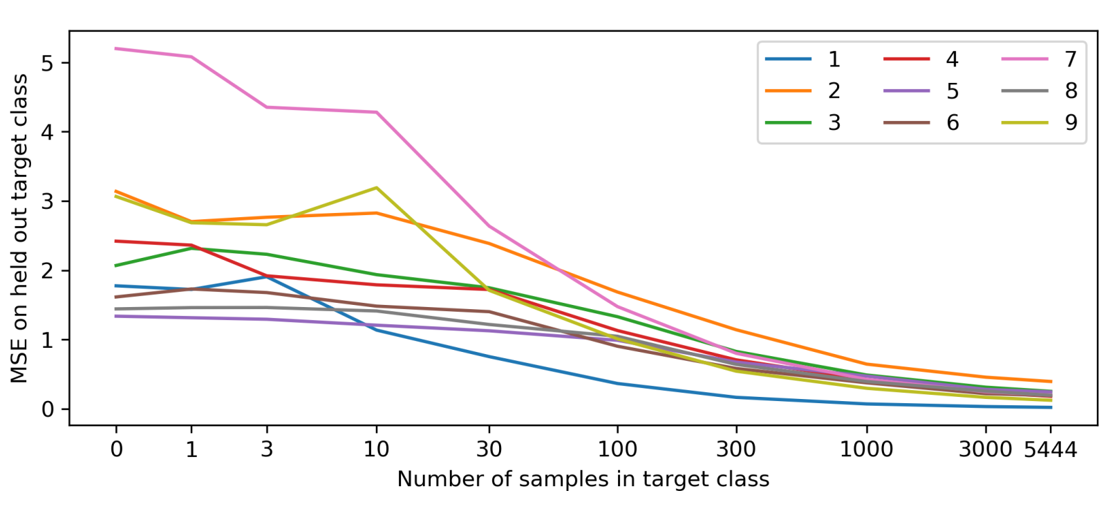
To test the validity of detecting novelty through the prediction error of target and predictor networks, we consider a toy model with MNIST. We train the predictor neural network on a mixed dataset of images with two classes: the 0 class and the target class (ex. 1). The 0 class represent states have been seen many times before, and the target class represent novel states. We vary the proportion of 0 class to target class while keeping the total amount of data constant, and see that the test error decreases when more target class data is available.
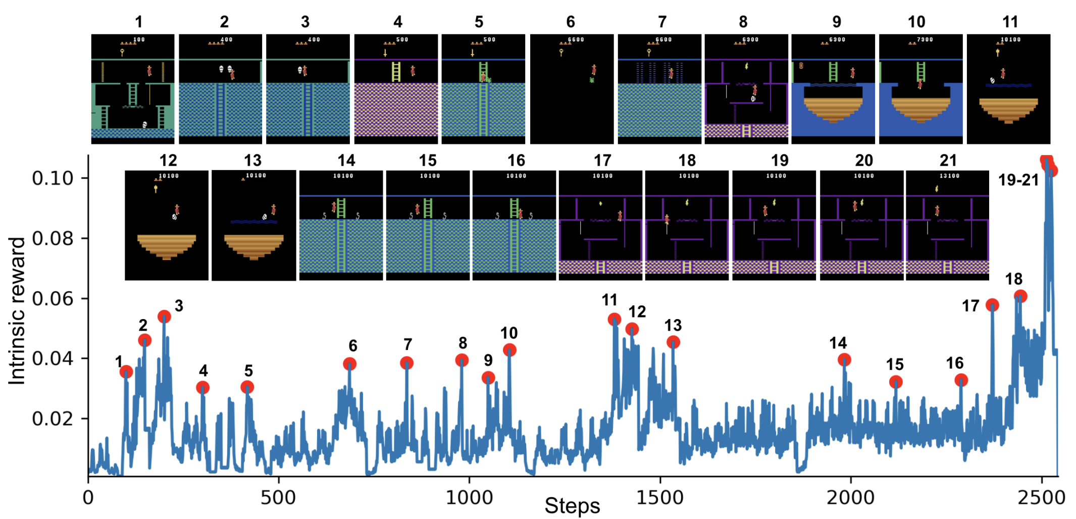
We also see empirically see that in Montezuma’s Revenge, the spikes in the intrinsic reward (or the prediction error) correspond to meaningful events: losing a life (2, 8, 10, 21), escaping an enemy by a narrow margin (3, 5, 6, 11, 12, 13, 14, 15), passing a difficult obstacle (7, 9, 18), or picking up an object (20, 21).
2.2.1 Sources of Prediction Errors
Generally, in deep learning, prediction error can be attributed to four factors:
- Amount of training data: Prediction error is high because the predictor fails to generalize from previous seen examples.
- Stochasticity: Prediction error is high because the prediction target is stochastic.
- Model misspecification: Prediction error is high because information necessary for prediction is missing, or because the predictor’s model is too limited to model the complexity of the prediction target.
- Learning dynamics: Prediction error is high due to failing to find the best approximation of the prediction target in the optimization process.
Factor 1 is a useful source of error, since it validates the use of RND. However, other sources of prediction errors can create undesirable effects in prediction-based exploration methods.
The most famous example is the noisy-TV problem, relevant to factor 2. Consider a maze environment with visual input. In this deterministic environment, maximizing prediction error would be beneficial, since it rewards exploring unvisited areas. Now, suppose there is a noisy TV attached to a wall inside the maze. Now, if the agent ever looks at the TV, it will always receive high reward, due to its randomness.

Although this example might feel too artificial, prediction-based exploration was shown to be attracted to the inherent stochasticity of the environment. This includes Montezuma’s Revenge.

Previous methods tried to avoid these factors by using the relative improvement of the prediction error $\Delta E$, rather than the absolute error $E$. Sadly, this is difficult to implement efficiently. In contrast, RND obviates both factors 2 and 3. The target network is fixed, so it is deterministic, not stochastic. Also, the target network and the predictor network has the same architecture, so the model cannot be limited.
2.2.2 Relation to Uncertainty Quantification
It is possible to see the prediction error of RND as a quantification of uncertainty.
Consider a regression problem with the data distribution $D = \{x_i, y_i\} _ i$. In the Bayesian setting, we would consider a prior $p(\theta^* )$ over the parameters of a mapping $f_{\theta^*}$, then calculate the posterior after updating on the evidence.
We follow Lemma 3 of Osband et al. (2018).
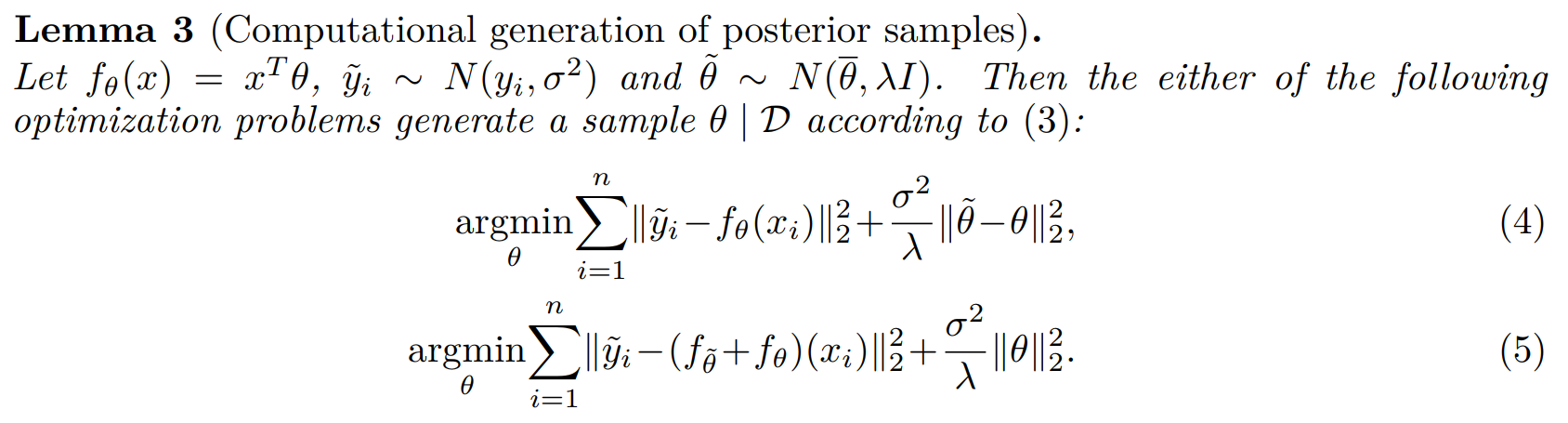
Let $\mathcal{F}$ be the distribution over functions $g_\theta = f_\theta + f_{\theta^* }$ (ensemble). $\theta^ *$ is drawn from the prior $p(\theta^ *)$, and $\theta$ is given by minimizing the expected prediction error \(\theta = \text{argmin}_ \theta \mathbb{E}_{(x_i, y_i) ~ D} || f_\theta(x_i) + f_{\theta^*}(x_i)-y_i||^2 + \mathcal{R}(\theta)\) where $\mathcal{R}(\theta)$ is a regularization term shown at the end of equations (4) and (5) of Lemma 3.
Now, let us confine the regression problem to predicting the constant zero function $y_i = 0$. \(\theta = \text{argmin}_ \theta \mathbb{E}_{(x_i, y_i) ~ D} || f_\theta(x_i) + f_{\theta^*}(x_i)||^2 + \mathcal{R}(\theta)\) Then, the optimization problem is equivalent to distilling a randomly drawn function from the prior. With $f_\theta^*$ being the target and $f_\theta$ being the predictor, the distillation error can be seen as a quantification of uncertainty in predicting the constant zero function $y_i = 0$.
2.3 Combining Intrinsic and Extrinsic Returns
Intrinsic Reward and Non-episodic Environment
When using only intrinsic reward, we explore changing the problem as non-episodic. In other words, we do not truncating the return when the game is over. There are several justifications for this. First, it tells the agent that its intrinsic return should be related to all the novel states that it could find in all future episodes, not just this episode. Also, using episodic intrinsic rewards can leak information about the task to the agent, so it no longer becomes intrinsic-only. (Burda et al., 2018)
We argue that this approach is also closer to how humans explore games. Suppose Alice is playing a tricky part of the game where it is easy to fail. If she succeeds, then she will fulfill her curiosity, so the reward is high. If she fails, she has to repeat “boring” task again, so the reward should be low. However, if Alice is modeled as an episodic agent, the return of game over is 0 by definition, which could be a high reward depending on the environment. Thus, in some environments, Alice will be overly risk-averse, not considering the “boredom” from game over.
For empirical results, check Section 3.1.
Extrinsic Reward and Episodic Environment
However, when we use extrinsic rewards, we should use the episodic problem setting. If we use non-episodic returns, the agent could find a strategy to exploit this setting by finding an extrinsic reward close to the beginning of the game and deliberately dying quickly. This can be seen as reward farming, a common phenomenon when the reward function is designed inappropriately.
Combining Intrinsic and Extrinsic Reward
Intrinsic rewards benefit from non-episodic setting, while extrinsic rewards benefit from episodic setting. We want a dense reward signal, so we want to use both intrinsic and extrinsic rewards, but it is nontrivial to to estimate the combined return from two streams of rewards.
We solve this by fitting two value heads $V_E$ and $V_I$ separately to their respective returns. $V_E$ estimates the cumulative extrinsic reward, while $V_I$ estimates the cumulative intrinsic reward. We then add these two value heads to get the value function $V = V_E + V_I$.
Fitting two value heads can have a bonus effect: the extrinsic reward function is stationary, while the intrinsic reward function is non-stationary. If we were to use a single value function $V$, it would need to estimate a non-stationary reward function. However, with two value heads, $V_E$ can focus on the stationary reward function.
For empirical results, check Section 3.2.
Separate Value Functions
We discussed fitting two value heads above in the context of combining two reward streams with different problem setting. However, the same idea can also be used to combine reward streams with different discount factors $\gamma$.
For empirical results, check Section 3.3.
3 Experiments
3.1 Pure Exploration
In Section 2.3, we argued that when we only use the intrinsic reward $i_t$, the non-episodic setting is a more natural setting. We empirically test this assumption by training agents on Montezuma’s Revenge. We use two metrics: mean episodic return and mean number of rooms found.
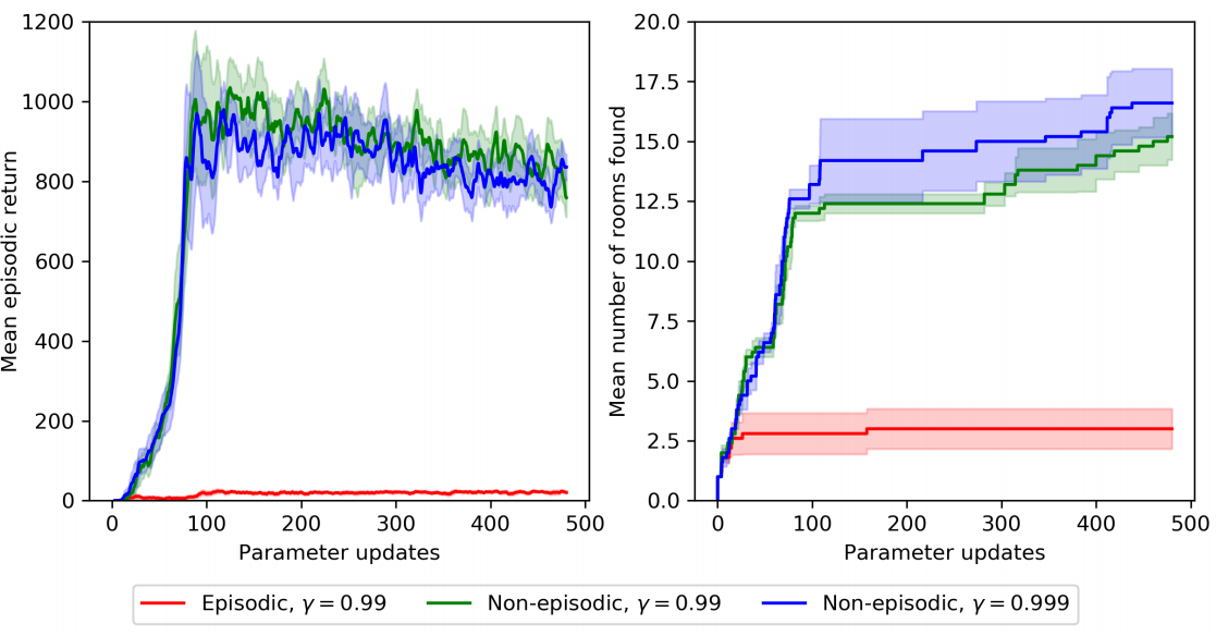
Since the agent is using the intrinsic reward only, it is not directly optimizing for either metric. However, to get high intrinsic reward, the agent needs to find novel states, including finding the key and opening the room with that key. Thus, we do see an improvement over time in both metrics.
Note that the mean episodic return are somewhat inconsistent. This is because once the agent learned how to use an item or reach a room, it is no longer interesting to the agent, so the intrinsic reward of performing such actions is low.
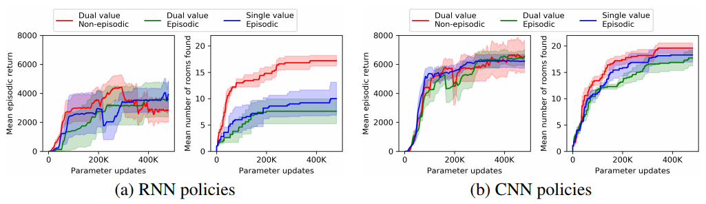
3.2 Combining Episodic and Non-episodic Returns
In Section 3.1, we compared episodic and non-episodic setting using only the intrinsic rewards. Now, we compare these settings again using both intrinsic and extrinsic rewards. We fix extrinsic rewards to be episodic and compare episodic and non-episodic settings for the intrinsic rewards. We also include the results of using a single value head if both rewards are episodic.
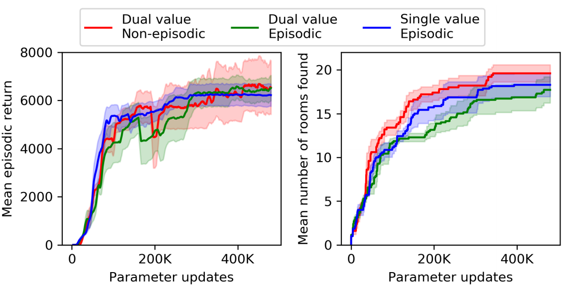
Contrary to our expectations, using two value heads with non-episodic intrinsic reward and episodic extrinsic reward did not show any benefit over other methods. Nevertheless, we will use two value heads with non-episodic intrinsic reward for the rest of the experiments.
3.3 Discount Factors
Previous state of the art works of Montezuma’s Revenge reported better performance using higher discount factor, since it allows the agent to look further into the future. Thus, we compare different values of $\gamma_I, \gamma_E$.
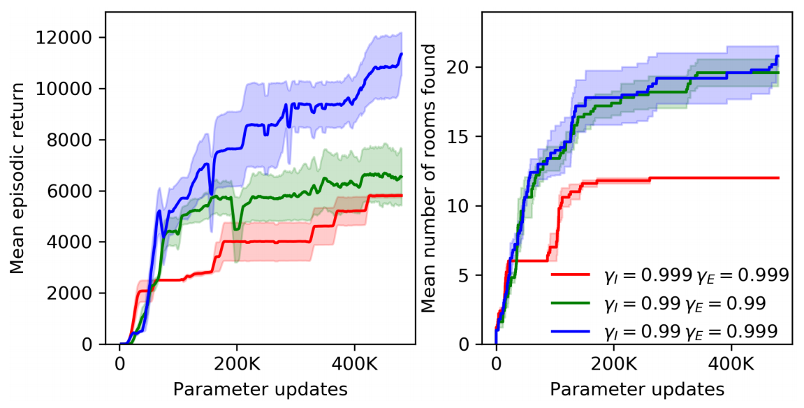
We see that $\gamma_I = 0.99$ and $\gamma_E = 0.999$ yields best result, with a mean return of 11.5K.
3.4 Recurrence
Montezuma’s Revenge is a partially observable environment. The observation only include information about the current room and the number of keys the player has. From the observation, the agent cannot deduce where the keys came from, how many were used, or which doors are open.
To deal with this partial observability, it is possible to reformulate a state as a summary of the past using a recurrent neural network (RNN). This is a similar approach to deep recurrent Q-network (DRQN).
We call the new state formulation the RNN policy, and call the old state formulation using just the visual observation the CNN policy.
Contrary to our expectation, RNN policy results in a worse performance compared to CNN policy.
3.5 Scaling Up RNN Training
In this section we further investigate RNN policies to show the effect of increased scale of parallel environments. For all experiments in this section, intrinsic rewards are non-episodic, and $\gamma_I = 0.99, \gamma_E = 0.999$.
We test $[32, 128, 256, 1024]$ number of parallel of environments. For a fair comparison of environments, we need to fix the batch size. This is because having a larger batch size results in the predictor network learning quickly, resulting in a rapid decrease in the intrinsic reward function. Thus, when we scale up from 32 environments to 128, we randomly drop out 75% of the elements, keeping just 25%. Similarly, when we scale up from 32 to 256 and 1024, we keep just 12.5% and 3.125% of the batch.
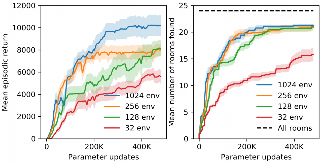
As predicted, we see that the agent performs better with more parallel environments. With 1024 environments, the RNN RND agent had a mean episodic return of 10070 with the best return of 14415.
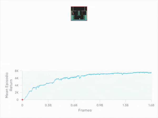
Separately, we allowed the the RNN RND agent with 32 environments to train for 1.6M parameter updates (1.6B frames). This agent had a mean episodic return of 7570, and the best run was able to achieve a return of 17500, visiting all 24 rooms and completing the first level.
3.6 Comparison to Baselines
We now compare RND to two existing works on 6 hard exploration Atari 2600 games: Gravitar, Montezuma’s revenge, Pitfall!, Private Eye, Solaris, and Venture.
The first baseline is the “vanilla” PPO, without any exploration bonus.
The second baseline is PPO with a different exploration bonus mechanism based on forward dynamics error. There are numerous works on designing intrinsic rewards with forward dynamics. Among those, we selected the Intrinsic Curiosity Module (ICM) used in by Pathak et al. (2017) and Burda et al. (2018). It is a good representative of prior methods using forward dynamics error.
Furthermore, Burda et al. showed that training a forward dynamics model in a random feature (RF) space works as well as any other feature space most of the time, so we can use the RF space instead (ICM-RF). RND and ICM-RF is quite similar, allowing for a direct comparison on algorithms while fixing other part of the methods such as dual value heads, non-episodic intrinsic returns, normalization schemes, etc.
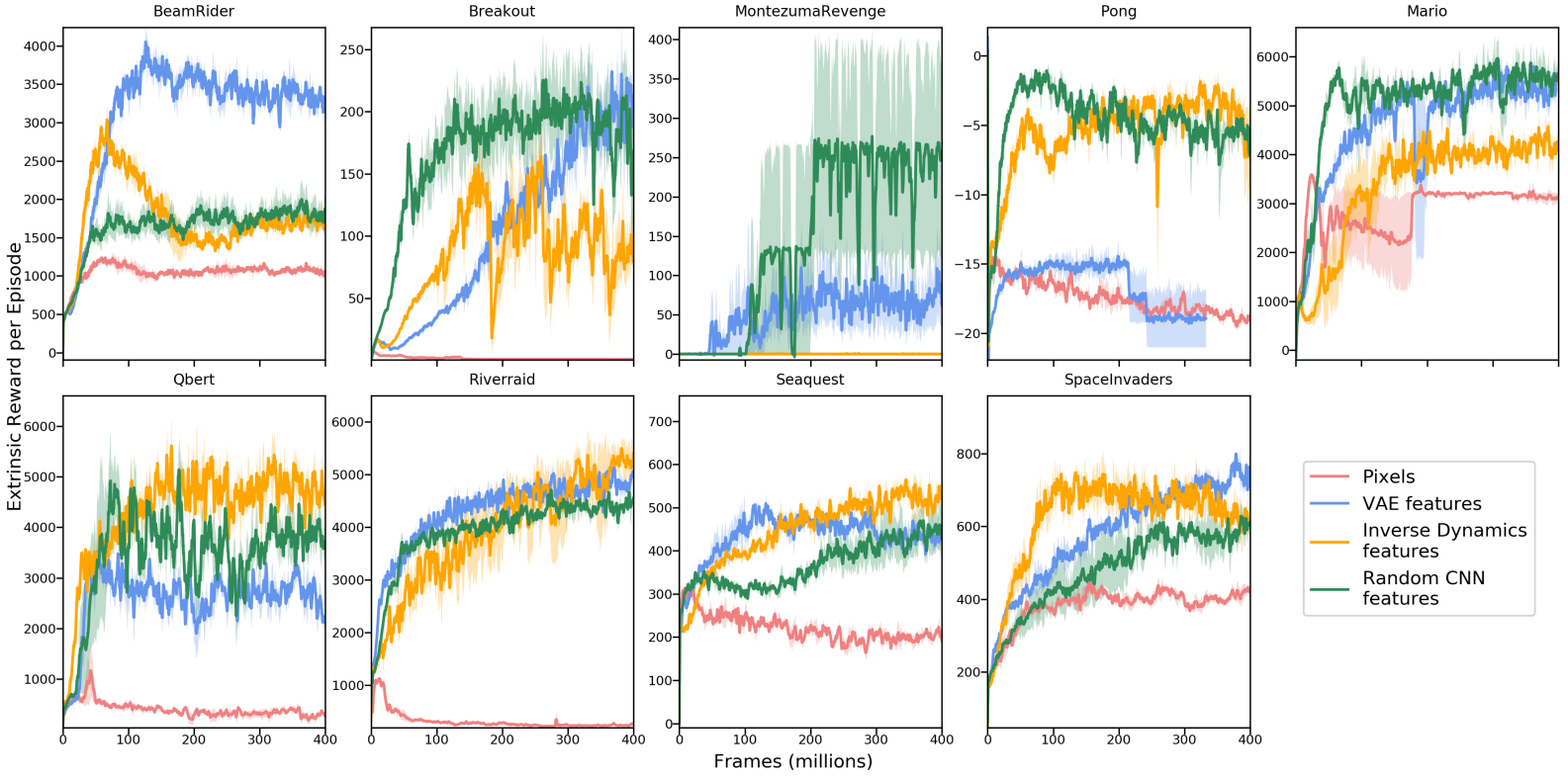
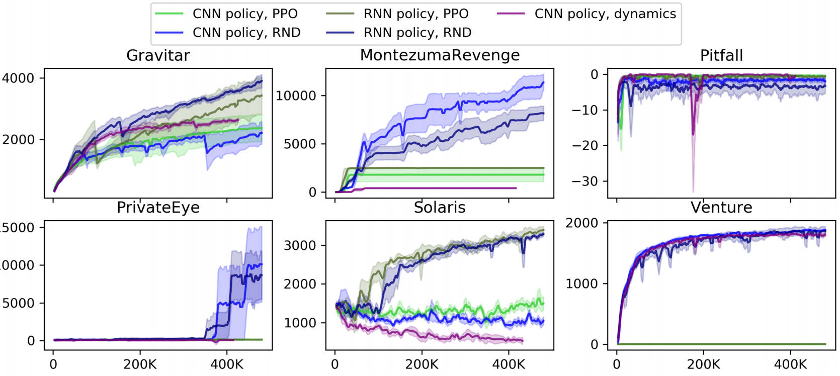

RND achieves new SotA for Gravitar and Montezuma’s Revenge and competes SotA in Venture. RND gets a sub-SotA score on Private Eye and Solaris but is better than PPO and ICM-RF. Like all other methods, RND fails to get positive score for Pitfall.
3.7 Qualitative Analysis: Dancing with Skulls
Observing the RND agent, we found that once the agent obtains all the extrinsic rewards it knows how to obtain reliably, it continues to interact with potentially dangerous objects. For instance, in Montezuma’s Revenge, the agent jumps back and forth over a moving skill that upon contact makes agent lose life. Similarly, in Pitfall, the agent repeatedly “dances” with the rope and the scorpion.
We speculate that the agent adapts this behavior because such dangerous states are difficult to achieve or stay alive, it is therefore rarely represented in the agent’s past experience compared to safer states.
4 Related Work
4.1 Exploration
There are a lot of previous works on exploration, categorized in three broad classes.
Count-based exploration are exploration methods that “count” the number of times each state was visited and defines a decreasing exploration bonus with respect to the visitation count. For high-dimensional state spaces where most states are visited only once, methods such as “pseudo-counts” are devised using density models to generalize the concept.
Dynamics prediction methods are exploration methods that predict the environment dynamics and use the prediction error to define the exploration bonus. Simply using the prediction value makes the agent susceptible tho the “noisy-TV” problem in stochastic or partially observable environment, so different metrics such as measuring prediction improvement is used.
Other exploration methods include adversarial self-play, empowerment maximization, parameter noise injection, option discovery, and ensembles.
4.2 Montezuma’s Revenge
Commonly known as one of the hardest problem of Atari 2600 since the birth of DQNs, Montezuma’s Revenge has been a standard benchmark for exploration algorithms.
Without any explicit exploration bonus, early deep reinforcement learning algorithms such as DQNs failed to make meaningful progress. However, in 2018, Ape-X, IMPALA and SIL showed that even without such bonus, it is possible to achieve a score of 2500.
Using pseudo-count exploration bonus discussed above allowed for new state of the art performance, as shown by DQN-CTS and DQN-PixelCNN.
Some have also improve exploration by using the internal RAM state available, hand-crafting exploration bonuses. Despite such access, these methods still achieved below the score of an average human.
Expert demonstrations have been used to simplify the exploration problem. With this information, multiple methods such as atari-reset achieved superhuman performance. However, learning from expert demonstrations exploits the deterministic nature of the environment. To prevent the agent from simply memorizing the expert’s sequence of actions, newer methods have been tested with the stochastic variant with sticky actions (each action repeated with some probability).
4.3 Random Features
Using the features of a random initialized neural network have been extensively studied in the context of supervised learning. It has also recently been used in reinforcement learning as an exploration technique by Osband et al. (2018) and Burda et al. (2018). This work was motivated by Osband et al. as shown in Section 2.2, and the work of Burda et al. was used as a baseline in Section 3.6.
4.4 Vectorized Value Functions
The idea of a vectorized value function was used in Temporal Difference Models (TDM; Pong et al.,2018) and C51 (Bellmare et al., 2017).
5 Discussion
We introduced a new exploration method based on random network distillation and showed its capability through Atari 2600 games with sparse rewards. RND was able directed exploration to achieve high performance despite its simplicity. This suggests that when applied at scale, even simple exploration methods can solve hard exploration games. The results also suggest that methods that can treat intrinsic and extrinsic rewards separately can benefit from such flexibility.
We find that RND is enough to deal with local exploration: exploring the consequences of short-term decisions, like choosing to interact or avoid a particular object. However, global exploration that involves coordinate decisions over long time horizons is beyond our reach.
For example, let us consider Montezuma’s Revenge. The RND agent is good at exploring the short-term decisions: it can choose to use or avoid the ladder, key, skull, or other objects. However, Montezuma’s Revenge requires more than these local explorations. In the first level of Montezuma’s Revenge, there are four keys and six locked doors spread throughout the level. Any key can open any door, but is consumed in the process. To solve the first level, the agent must enter a room locked behind two doors, so the agent must not open the two other doors that are easier to find, even though they would be rewarded for opening them. This requires global exploration through long-term planning.
How can we convince the agent to make such behavior? Since not opening the other two doors results in a loss of rewards, the agent should receive enough intrinsic reward to compensate for the loss of extrinsic rewards. The RND agent does not seem to get enough incentive through intrinsic rewards to try this strategy, and thus it rarely manages to finish the level.
An important future work will be to devise a method that can solve similar problems that require high-level global exploration.
Final Thoughts
Questions
- The authors argue that RND trivializes the noisy-TV problem. However, can’t “dancing with skulls” be thought of as a variant of the noisy-TV problem?
- In simulated environments, “dancing with skulls” is just an interesting concept, but in mission-critical systems, it is a big threat. Are there some methods to make this agent more safe?
- In Section 5: Discussion, the authors argue that RND shows how dividing intrinsic and extrinsic rewards could benefit the agent. Isn’t this contrary to the experimental results?
Recommended Next Papers